
Applications gallery
The application examples from the original milamin.org: what MILAMIN’s mechanical, Stokes and thermal solvers were used for. The simulation videos stream from the original PGP Vimeo account, fifteen years on.
1. Rigid inclusions
Rigid Circular Inclusions Subject to Simple Shear
A Rigid Circular Inclusion in Anisotropic Host Subject to Simple Shear
We used MILAMINs fast MATLAB-based incompressible Stokes solver to study the flow around a circular rigid inclusion embedded in an anisotropic linear viscous matrix. A schematic representation of the studied model is presented in the figure below.
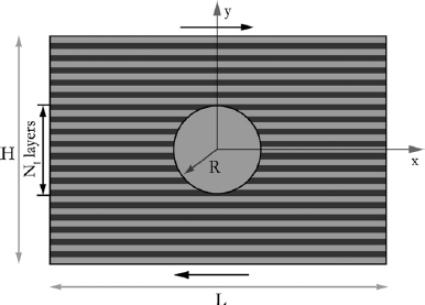
A schematic representation of the studied model. In the limit N -> infinity, the host is modeled as an anisotropic fluid. Constant horizontal velocity on the top and bottom walls is prescribed and periodic velocity is imposed on the lateral boundaries in numerical simulations.
Evolution of the structure and shear rate distribution with increasing shear strain are presented. The anisotropy factor is equal to 10. An arbitrarily spaced set of lines is used as passive markers for visualizing the structure.
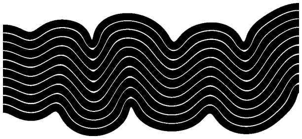
2. Multilayer folding
3. Sedimentation
Sedimentation
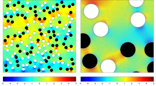
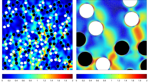
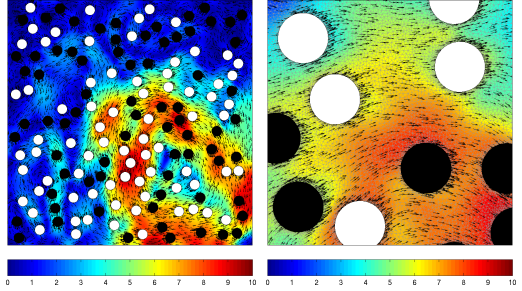
In this section we present the results of our sedimentation study, which is another application example of the MILAMINs mechanical solver. The circular deformable inclusions in a box are subjected to vertical gravity field. Black (heavy) and white (light) inclusions have the same density contrast with respect to the matrix. They are hundred times more viscous than the matrix. The color-scale represents the magnitude of the velocity field, with warm colors corresponding to high values and cold colors to low values.
In the following movie we present results from a sedimentation study with rigid inclusions shaped as ellipses.
We also present results from a sedimentation study with rigid circular inclusions with varying sizes.
4. Thermomechanical modeling
We have devised a numerical tool for studying processes that take place in the deeper mantle, using MILAMINs fast MATLAB-based Stokes and thermal solvers.
A thermomechanical Finite Element Method (FEM) code is developed to model convection of a viscous fluid in a rectangular domain. The fluid is confined in an impermeable box and is heated from below, with no internal heating. It is assumed that the fluid is of infinite Prandtl number, with Newtonian rheology and that the Boussinesq approximation applies. The fluid is comprised by two chemically distinct materials: a dense layer along the bottom boundary overlain by a material of lower density and higher viscosity. Density and viscosity of the entire fluid are both temperature- and chemistry-dependent. Mechanical boundary conditions are free slip on all four sides of the box. Thermal boundary conditions are isotherms on top and bottom boundaries and zero heat flux on lateral boundaries.
The governing equations include the conservation laws of mass, energy, and momentum, as well as the thermal and chemical dependence of viscosity. Density variations are expressed as a linear combination of thermal and chemical contributions.
Two independent grids are used for spatial discretization of the temperature and velocity fields. We use a structured grid, and the resolution is determined by the number of mechanical elements in vertical direction and the number of thermal elements per mechanical element. Different materials in the model are represented by markers, and material transport associated with convection is modeled using marker-in-cell technique.
Temporal evolution of the temperature field and distribution of the dense layer are presented below. The resolution is determined by 100 mechanical elements in vertical direction and 2×2 thermal elements per mechanical element. We use second order quadratic elements for the velocity, and first order quadratic elements for the temperature.